Mapping the Geometry of Growth

The Laplace transform is a mathematical bridge. It takes time-domain functions and maps them to the complex s-plane. Here, every point represents a function of the form e to the st.
Imagine growth, decay, and oscillation as coordinates. The imaginary axis handles the rhythm, while the real axis dictates the scale. High imaginary values correspond to functions with more oscillation.
The s-plane is the ultimate atlas for dynamic behavior.
If a function has a negative real part, it decays toward zero. Conversely, positive real parts signal a system heading toward explosive instability. Engineers look for these signs to prevent disaster.
In nature, systems are rarely pure. They are combinations of growth and decay. Therefore, we need a tool that can isolate these components with surgical precision. This is why the Laplace transform is not just an equation, but a lens.
- Negative Real: Stable decay
- Positive Real: Unstable growth
- Imaginary Axis: Pure oscillation
- Complex Poles: Spiraling trajectories
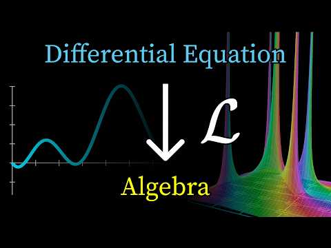
Turning Calculus into Simple Algebra

Differentiation is the traditional nightmare of engineering. But the Laplace transform changes the game entirely. It converts complex derivatives into basic multiplication. This is its most potent superpower.
Multiplying by s in the transform space is essentially the same as taking a derivative in time. However, there is a crucial correction term. You must subtract the initial condition f(0) from the result.
ここからが大事な
ポイントです
具体例・注意点・明日から使えるヒントを整理しています。
✨無料閲覧で全文 + 図解の完全版を3日間いつでも読み返せる
あなたの好きな動画も、
1分でAI要約
📚 お気に入り保存 + ✨ あなたの動画をAI要約
(無料登録10秒)
✏️ この記事で学べること
- ▸s
- ▸「」
10秒で完了・パスワード作成不要